Kimi K3 vs GLM-5.2 (2026): Frontier Worth 2.8x the Cost?
Kimi K3 ($3/$15/M) costs ~2.8x GLM-5.2 ($1.40/$4.40) per run but scores higher on Artificial Analysis (57 vs 51). When the premium pays, with worked math.
 Ofox
Ofox 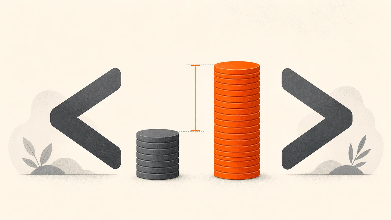
TL;DR. GLM-5.2 (z-ai/glm-5.2) is the cheaper model and Kimi K3 (moonshotai/kimi-k3) is the stronger one, and the gap in both directions is real. On ofox.ai K3 lists at $3/$15 per million against GLM-5.2’s $1.40/$4.40, so a typical run (50K input, 20K output, no cache) costs $0.45 on K3 vs $0.158 on GLM-5.2, about 2.8x more. For that premium, Artificial Analysis scores K3 higher on general intelligence (57 vs 51) and clearly higher on agentic tasks (GDPval v2 Elo 1668 vs 1514), and K3 adds native vision. Both are open weight and both share a 1M context, so GLM-5.2’s old context edge over Kimi is gone. The decision is simple to state and workload-specific to answer: pay 2.8x for K3 when the capability gap earns it, stay on GLM-5.2 when good-enough at a third of the cost wins.
This is an upgrade of an earlier cost comparison. Last cycle the cheaper Kimi (K2.7 Code) undercut GLM-5.2, and the story was “how much cheaper.” With K3 the arrow flips: Kimi is now the premium option, and the honest question is whether the frontier is worth the markup on your runs.
TL;DR: Which One Should You Pick?
| Scenario | Pick | Why |
|---|---|---|
| High-volume coding, quality already good enough | GLM-5.2 | ~1/3 the per-run cost, same 1M context |
| Agentic tool use, multi-step autonomy | Kimi K3 | +154 GDPval v2 Elo; the premium buys a measured gap |
| Screenshot / diagram / vision input | Kimi K3 | native vision; the GLM-5.2 route here is text-only |
| Whole-repo prompts near 1M tokens | Either | both are 1M now; decide on price vs capability |
| Self-host open weights today | GLM-5.2 | MIT weights are out; K3 weights land by July 27 2026 |
| Hardest reasoning where the ceiling matters | Kimi K3 | higher AA index and stronger science/agent benchmarks |
| You want to decide from real numbers | Run the A/B loop | token consumption per run is workload-specific |
The honest verdict: GLM-5.2 is the cost-sensitive default and Kimi K3 is the capability upgrade you buy deliberately. The per-run price favors GLM-5.2 at every mix; the benchmarks favor K3 at every measure. Where those two facts cross is your own quality bar, and the split above is where the money actually moves.
Quick Specs Comparison
Prices are ofox.ai gateway rates, USD per million tokens, read off the model catalog on July 17 2026. AA figures are a rolling snapshot around K3’s July 2026 launch.
| Spec | Kimi K3 | GLM-5.2 |
|---|---|---|
| ofox model ID | moonshotai/kimi-k3 | z-ai/glm-5.2 |
| Input price | $3.00 / M | $1.40 / M |
| Output price | $15.00 / M | $4.40 / M |
| Cache read price | $0.30 / M | $0.26 / M |
| Context window | 1M (1,048,576) | 1M (1,048,576) |
| Image input | Yes (native vision) | No (text route) |
| Architecture | MoE, 2.8T total | ~753B parameters |
| AA Intelligence Index | 57 | 51 |
| AA GDPval v2 Elo | 1668 | 1514 |
| Weights | Open, by July 27 2026 | Open, MIT (released) |
Two things to pull off this sheet before the math. GLM-5.2 is cheaper on all three billed axes, so any workload pays less per token on GLM-5.2. And the context windows are now equal at 1M, which removes the single biggest reason the older Kimi lost this comparison on large prompts. So the trade collapses to one axis: you are paying a price premium for a measured capability premium, and nothing else about the specs breaks the tie.
Per-Run Cost: K3 Is the Premium Option
Per-token prices are the inputs, not the answer. Run cost is price times tokens consumed. Take a representative agent run of 50K input tokens and 20K output tokens, no cache.
| Cost line | Kimi K3 | GLM-5.2 |
|---|---|---|
| Input (50K) | $0.150 | $0.070 |
| Output (20K) | $0.300 | $0.088 |
| Run total | $0.450 | $0.158 |
K3 costs about 2.8x the run. Most of that gap is the output line: K3’s $15/M output is 3.4x GLM-5.2’s $4.40/M, and a reasoning-heavy agent puts a lot of tokens through output. On this mix, output alone accounts for two-thirds of K3’s bill. That is the number to keep in mind for the cache and mix sections below, because it is what makes K3’s premium sticky.
The reason to run the arithmetic rather than eyeball the price sheet is that per-token price and per-run price rank the models the same way here but not by the same amount. GLM-5.2 is 53% cheaper on input and 71% cheaper on output per token, yet the run comes out 65% cheaper, because the run weights the axes by how many tokens actually flow through each. Change the mix and the run gap changes with it, even though the sticker prices do not move. So a decision made off the specs table alone will be directionally right and quantitatively wrong, and at volume the quantity is the whole point.
What the Premium Buys
If K3 cost the same as GLM-5.2, this would be no contest. It does not, so the question is what the 2.8x buys. Three single-source reads from Artificial Analysis, so the comparison stays honest.
| Measure (Artificial Analysis) | Kimi K3 | GLM-5.2 |
|---|---|---|
| Intelligence Index | 57 | 51 |
| GDPval v2 agentic Elo | 1668 | 1514 |
| Cost per task | $0.94 | $0.32 |
On general intelligence K3 is six points up. On the GDPval v2 agentic evaluation, which scores realistic multi-step tool-use work rather than trivia, K3 leads by 154 Elo, a wider margin than the index gap suggests. That tracks with K3 taking the top spot on AA’s AutomationBench workflow eval. The third row is the honest counterweight: AA’s own cost-per-task measure has K3 at $0.94 against GLM-5.2’s $0.32, roughly the same 2.9x you see in the per-run math, so the capability gain and the cost are proportional. You are not overpaying for K3, but you are not getting a discount either. It is a straight quality-for-money trade.
There is one effect that works in K3’s favor on the money. A stronger model can sometimes finish a task in fewer tokens, and Artificial Analysis noted K3 used about 21% fewer output tokens than the previous Kimi generation to complete their index. Since the run bill is price times tokens, fewer tokens partly offset the higher per-token rate. But do not over-count it: AA’s cost-per-task figure already bakes token consumption in, and it still lands at $0.94 versus $0.32, a 2.9x gap that matches the per-run math. So on these workloads token efficiency trims the edges, it does not close the gap.
One discipline note. These AA numbers and any Moonshot- or Zhipu-reported benchmarks are different measurement systems. The rows above all come from Artificial Analysis so they are comparable to each other. Do not line them up against a vendor’s own published score from a different harness.
Cache Impact: The Premium Grows, It Does Not Shrink
Caching discounts input tokens only. Because K3’s disadvantage is concentrated on output, a higher cache-hit rate makes output a larger share of the bill and pushes the ratio the wrong way for K3.
| Input cache hit | Kimi K3 run | GLM-5.2 run | K3 / GLM |
|---|---|---|---|
| 0% | $0.450 | $0.158 | 2.85x |
| 50% | $0.383 | $0.130 | 2.95x |
| 80% | $0.342 | $0.112 | 3.04x |
This is the opposite of the older Kimi-vs-GLM story, where caching ate the cheaper model’s edge. Here, the more you cache, the more K3’s output-heavy pricing dominates, so the premium creeps from 2.8x toward the raw output ratio of 3.4x. If your workload is a high-cache code-review loop, K3 is not just pricier, it is relatively pricier than the headline suggests.
Mix Sensitivity and Volume
The ratio also moves with the shape of the traffic. Input-heavy runs pull toward the input ratio of 2.1x ($3.00 vs $1.40); output-heavy runs pull toward the output ratio of 3.4x. So across realistic workloads K3 runs roughly 2.1x to 3.4x the cost of GLM-5.2, with the 50K/20K case landing near the middle at 2.8x.
At volume, that middle case is a real line item. Here is the same 50K/20K run scaled up.
| Runs / month | Kimi K3 | GLM-5.2 | K3 extra |
|---|---|---|---|
| 1,000 | $450 | $158 | $292 |
| 5,000 | $2,250 | $790 | $1,460 |
| 20,000 | $9,000 | $3,160 | $5,840 |
At a thousand runs a month the difference is $292, about $3,500 a year. At twenty thousand runs it is $5,840 a month, the price of a headcount decision rather than a rounding error. That is the weight on the GLM-5.2 side of the scale. The weight on the K3 side is the 154-Elo agentic gap and vision, which either matters for your tasks or does not. The tables cannot make that call for you; they only make the cost of the call explicit, so that when you route bulk traffic to one model or the other you are doing it with the annual number in view.
flowchart TD
    A[Agent run] --> B{Needs vision or hardest agentic quality?}
    B -->|Yes| C[Kimi K3<br/>moonshotai/kimi-k3]
    B -->|No| D{High volume and quality already good enough?}
    D -->|Yes| E[GLM-5.2<br/>z-ai/glm-5.2<br/>~1/3 the per-run cost]
    D -->|No| F{Is the 154-Elo agentic gap worth ~2.8x?}
    F -->|Yes| C
    F -->|No| E
The Token-Consumption Wildcard
Every number so far assumes the two models emit the same tokens for the same task. They will not. Run cost is price times tokens, and the second factor is model-specific: a model that plans efficiently can finish in fewer output tokens, while one that rambles or retries burns more. That matters here because output is where K3’s premium concentrates. If K3 completes an agent task in meaningfully fewer output tokens than GLM-5.2, its effective per-task premium is smaller than the 2.8x the price sheet implies. If it thinks longer on max effort, the premium is larger.
The price side is exact, taken from the ofox catalog. The token side is not something I can compute for your tasks, because no one has published a first-party token-consumption benchmark on identical agent runs for these two models, and it would be workload-specific even if they had. AA’s cost-per-task ($0.94 vs $0.32) is the closest normalized proxy, and it says the gap holds at roughly 2.9x across their suite. But your traffic is not their suite. The only way to settle it is the A/B loop below: run both on your real tasks, read the usage field, and let your own token counts answer the per-run question. Everything above tells you where to expect the answer to land; only your logs tell you where it actually does.
When to Pick Kimi K3
Pay the premium when the capability shows up in your output, not by default:
- Agentic and tool-use workloads. The 154-Elo GDPval v2 gap and the AutomationBench top spot are exactly the kind of multi-step autonomy where a weaker model wastes tokens flailing. Here K3’s higher price can even pay for itself in fewer retries.
- Vision tasks. Screenshots, diagrams, UI bugs. K3 takes image input natively; the GLM-5.2 route in this comparison is text-only.
- Hardest reasoning. Where the six-point intelligence gap changes whether the task completes correctly, not just faster.
The through-line: K3 earns its price when the task is hard enough or agentic enough that a weaker model would fail, retry, or need a human to clean up. Those failure costs do not show up on the API invoice, but they are real, and once you count the whole loop a model that gets it right the first time can be cheaper than a model that is cheaper per token. If your agent runs unattended, weight that heavily.
When to Pick GLM-5.2
Stay on the cheaper model when good-enough clears the bar:
- High-volume, cost-sensitive coding. At about a third of the per-run cost with the same 1M context, GLM-5.2 is the default for bulk work.
- Input-heavy, output-light jobs. RAG, summarize, classify. The output line where K3 is 3.4x pricier is small, but so is the reason to pay for it.
- Self-hosting today. GLM-5.2’s MIT weights are already out; K3’s are promised by July 27 2026 but not released yet.
The through-line: GLM-5.2 wins whenever the quality difference does not change the outcome, and most production coding traffic is routine. The efficient pattern is not “pick one model,” it is tiered routing: default bulk traffic to GLM-5.2, promote only the hard, agentic, or vision slices to K3. Because both share one ofox endpoint and one API key, that routing is a per-request string choice, not an integration project, so you can capture most of K3’s capability while paying GLM-5.2’s rate on the majority of calls.
When Neither Is the Right Call
If the job is text-only budget coding and you do not need GLM-5.2’s full 1M context, a smaller, cheaper Kimi may beat both on cost. Kimi K2.7 Code (moonshotai/kimi-k2.7-code) runs $0.95/$4 with a 256K context. At the extreme-budget end, Artificial Analysis lists DeepSeek V4 Pro at $0.04 per task, a fraction of GLM-5.2’s $0.32, though it trails on the intelligence index (44 against GLM-5.2’s 51), so it is the pick only when cost dominates every other consideration and the quality floor is low. And if you need the absolute top of the board rather than the value or the volume pick, the closed frontier (GPT-5.6 Sol, Claude Fable 5) sits above both K3 and GLM-5.2 on the AA index, at a price above both. For a wider view, see the real-use coding model ranking and the API pricing comparison.
Try Both via ofox: A/B in One Loop
Both models sit on the same OpenAI-compatible endpoint, so a real per-run comparison on your own task is a one-string swap. Point the SDK at https://api.ofox.io/v1, loop over the two model IDs, and read usage and latency. Grab a key on the ofox model page for Kimi K3.
Python: A/B both models in one loop
from openai import OpenAI
import os, time

client = OpenAI(base_url="https://api.ofox.io/v1", api_key=os.environ["OFOX_API_KEY"])

prompt = "Refactor this module for async I/O and add early returns on empty input: ..."

for model in ["moonshotai/kimi-k3", "z-ai/glm-5.2"]:
    t0 = time.time()
    resp = client.chat.completions.create(
        model=model,
        messages=[{"role": "user", "content": prompt}],
    )
    dt = time.time() - t0
    u = resp.usage
    print(f"{model}: {dt:.1f}s  in={u.prompt_tokens} out={u.completion_tokens}")
Node: same shape
import OpenAI from "openai";

const client = new OpenAI({
  baseURL: "https://api.ofox.io/v1",
  apiKey: process.env.OFOX_API_KEY,
});

const prompt = "Refactor this module for async I/O and add early returns on empty input: ...";

for (const model of ["moonshotai/kimi-k3", "z-ai/glm-5.2"]) {
  const t0 = Date.now();
  const resp = await client.chat.completions.create({
    model,
    messages: [{ role: "user", content: prompt }],
  });
  const dt = ((Date.now() - t0) / 1000).toFixed(1);
  const u = resp.usage;
  console.log(`${model}: ${dt}s  in=${u.prompt_tokens} out=${u.completion_tokens}`);
}
K3 only: attach a screenshot
K3 takes image input; the same call to z-ai/glm-5.2 on the text route fails. Send the image as an image_url block.
import base64

with open("layout-bug.png", "rb") as f:
    b64 = base64.b64encode(f.read()).decode()

resp = client.chat.completions.create(
    model="moonshotai/kimi-k3",
    messages=[{
        "role": "user",
        "content": [
            {"type": "text", "text": "This UI screenshot has a layout bug. What is wrong and how do I fix the CSS?"},
            {"type": "image_url", "image_url": {"url": f"data:image/png;base64,{b64}"}},
        ],
    }],
)
print(resp.choices[0].message.content)
Run the loop on a representative slice of your real tasks, sum usage across a day, and multiply by the specs-table prices. Token consumption per task is workload-specific and no leaderboard measures it for your traffic, so this loop is the only honest input to the per-run decision.
Cost per run and cost per million are different questions. The pricing index maps the six mechanisms between them.
FAQ
Is Kimi K3 more expensive than GLM-5.2? Yes. K3 is $3/$15/M vs GLM-5.2’s $1.40/$4.40/M. On a 50K/20K no-cache run that is $0.45 vs $0.158, about 2.8x. K3’s output price is 3.4x GLM-5.2’s, which is most of the gap.
Is Kimi K3 better than GLM-5.2? On Artificial Analysis, yes: 57 vs 51 on the Intelligence Index and 1668 vs 1514 on GDPval v2 agentic Elo, plus native vision. K3 is a 2.8T model, GLM-5.2 is 753B. Stronger, but about 2.8x the per-run cost.
Does the K3 premium grow or shrink with cache? It grows. Caching discounts input only, and K3’s disadvantage is on output, so more cache pushes the ratio from about 2.8x toward the 3.4x output ratio.
Which has the bigger context window? They tie at 1M tokens. The older Kimi K2.7 Code was 256K, so GLM-5.2 no longer has a context edge over the current Kimi flagship.
Are both open weight? GLM-5.2 ships MIT weights today (~753B). K3 is announced open weight with a release by July 27 2026 (2.8T), not out yet, so today it is API-only.
When should I pick GLM-5.2 over Kimi K3? For high-volume work where quality is already good enough. GLM-5.2 runs at about a third of the cost with the same 1M context. Reserve K3 for agentic, vision, or hardest-reasoning tasks where the gap changes the outcome.
Can I A/B both behind one key?
Yes, both are on api.ofox.io/v1 under the OpenAI-compatible protocol. Swap moonshotai/kimi-k3 for z-ai/glm-5.2 with the same key and SDK.
Sources Checked for This Refresh
Frequently Asked Questions
- Is Kimi K3 more expensive than GLM-5.2?
- Yes, by a lot. On ofox.ai, Kimi K3 is $3.00/M input, $15.00/M output, $0.30/M cache read. GLM-5.2 is $1.40/M input, $4.40/M output, $0.26/M cache read. On a typical run (50K input, 20K output, no cache) K3 costs $0.45 and GLM-5.2 costs $0.158, so K3 is about 2.8x the price per run. K3's output token price is 3.4x GLM-5.2's, which is where most of the gap lives.
- Is Kimi K3 better than GLM-5.2?
- On Artificial Analysis it scores higher: 57 vs 51 on the Intelligence Index, and 1668 vs 1514 on the GDPval v2 agentic Elo. K3 is a 2.8T model with native vision; GLM-5.2 is a 753B text model. So K3 is measurably stronger, especially on agentic tasks, but you pay roughly 2.8x per run for it. GLM-5.2 is the value pick, K3 the premium one.
- Does the K3 premium grow or shrink with cache?
- It grows. Because K3's biggest disadvantage is on output tokens (3.4x GLM-5.2's rate) and caching only discounts input, a higher cache-hit rate makes output a larger share of the bill and pushes the ratio up. On the 50K/20K run the ratio goes from about 2.8x at no cache to roughly 3.0x at 80% input cache. Cache does not help K3 catch GLM-5.2 on cost.
- Which has the bigger context window, K3 or GLM-5.2?
- They tie. Both offer a 1M-token context window (1,048,576 tokens). That is a change from the older Kimi K2.7 Code, which was 256K, so GLM-5.2 no longer has a context advantage over the current Kimi flagship. Choose on price and capability, not context size.
- Are both Kimi K3 and GLM-5.2 open weight?
- GLM-5.2 ships MIT-licensed open weights today (roughly 753B parameters). Kimi K3 is announced as open weight with a release by July 27 2026, and at 2.8T parameters it would be the largest open-weight model on the Artificial Analysis leaderboard once out. As of this writing K3's weights are not released yet, so today it is an API-only model.
- When should I pick GLM-5.2 over Kimi K3 on cost grounds?
- When your workload is high-volume and quality is already good enough, GLM-5.2 does the job at about a third of the per-run cost with the same 1M context. Route cost-sensitive bulk work there. Reserve K3 for tasks where the measured capability gap (agentic tool use, hardest reasoning) or vision input actually changes the outcome.
- Can I A/B both models behind one API key?
- Yes. Both are on api.ofox.io/v1 under the OpenAI-compatible protocol. Swap the model string from moonshotai/kimi-k3 to z-ai/glm-5.2 with the same key and SDK. The A/B loop at the end prints each model's latency and token usage per request, which is the only honest input to a per-run cost decision.